In the previous post I tried to summarize the Autobahn paper but its goal, seamlessness, seem convoluted. In this post, I will try to explain it in my own way so that hopefully it can be easier to understand and get myself an internship at Ethereum Foundation 🙂
Background & Motivation
We assume $f$ faulty validators and a total of $n=3f+1$ validators. We will still start by defining blips.
Blip: a period during which protocol does not make progress. This include network asynchrony, Byzantine leader elected, etc.
Existing practical BFT protocols can be largely categorized as partially synchronous and asynchronous, depending on their network assumptions. Traditional wisdom says that partially synchronous protocols deal poorly with blips. Asynchronous protocols can handle blips well as they proceed at network rate, but perform poorly during good periods due to excessive amount of message exchanges requred to ensure consensus. So this paper asks: why do partially synchronous protocols deal with blips so poorly? Can they do better?
Hangovers
Hangover: performance degradation caused by blips that lasts after blips end
Since no protocol can make progress during blips, the previous question can be rephrased as, why do partially synchronous protocols experience more serious hangovers than asynchronous protocols and how can we mitigate hangovers.
Take HotStuff as an example, after blips end and timeouts expire, a new benign leader is elected. It will batch client requests into a block, send the block out, collect votes, and send the collected votes with the next block of client requests. Since there are requests coming in during blips, new requests received after blips need to be queued after the old requests, leading to hangovers. So the key to the previous question is, how can we process requests accumulated during blips as fast as possible?
Separate Block Dissemination from Consensus
One existing technique is to separate block dissemination (sending block to other validators) from consensus ordering. The key observation is that consensus messages are often small, whereas blocks themselves are orders of magnitude larger, so removing block dissemination from consensus cirtical path can significantly reduce latency. Aptos, for example, uses Narwhal for block dissemination and Jolteon for consensus.
Autobahn similarly adopts this technique. It has an asynchronous block dissemination layer that ensures blocks can be disseminated even during blips and a consensus layer to pick from these blocks for ordering. However, in a naive implementation, since validators need to possess the blocks proposed by the leader before voting, the leader must pick blocks that all $2f+1$ benign validators have received, or they will request the blocks from peers before voting, moving block dissemination back onto the critical path. Yet a block dissemination layer that guarantees this inevitably require numorous message exchanges. Can we do better?
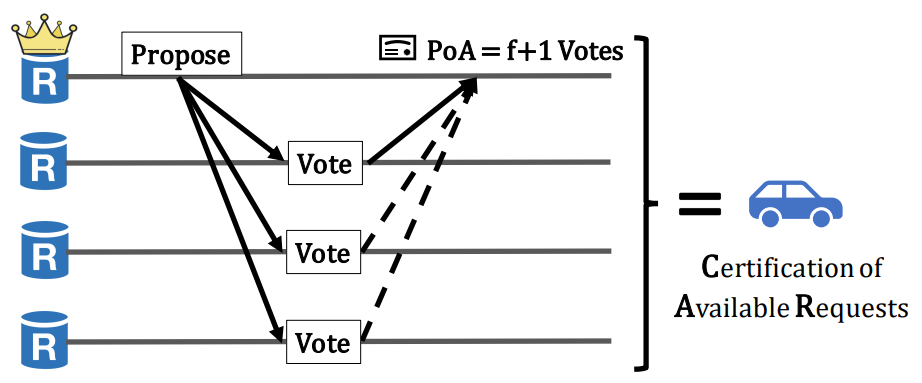
Proof of Availability (PoA)
Turns out validators do not need to validate the exact requests in blocks during consensus ordering – they can ignore bad requests during execution. So a benign validator can vote if the leader can convince it that the blocks will be available when needed. This weak guarantee only requires one benign validator to persist the block and use collision resistant hashes to ensure Byzantine validators cannot lie about block content. To provide this guarantee, during block dissemination, each validator will broadcast its blocks and wait for $f+1$ votes from peers, which it will combine to form a Proof of Availability (PoA). This process is called Certification of Availability Requests (CAR).
Certification of Available Requests
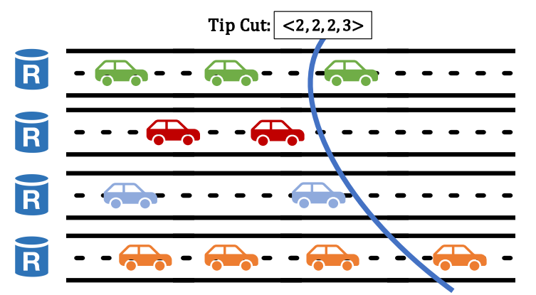
In Autobahn, validators broadcast blocks with the PoA of its parent block, forming a chain. This chain of CARs is called a lane and the last poposed block in a lane is called a tip. Each validator has its own lane. Byzantine validators may not always append new blocks to lane tip, leading to forks. Benign validators will only vote for a block if it has previously voted for its parent and it has not voted for another block by the same proposer at the same height. This way, PoA for one block proves the availability of all its ancestors.
However, since PoA only require $f+1$ votes, there can be blocks with PoAs at the same height and lanes can diverge. The consensus layer will choose one branch to commit.
Consensus
Autobahn can choose any BFT protocol for its consensus. The key is to include as much PoA as possible in the leader’s proposal. Once validators agree on the set of blocks to commit, they can locally decide how these blocks should be ordered locally through some deterministic algorithms.
Validators each manage a local view of all lanes. The leader will pick out the last certified tip (tip with a matching PoA) of every lane in its local view, forming a tip cut. The leader will include this tip cut in its proposal.
Lanes and Tip Cut
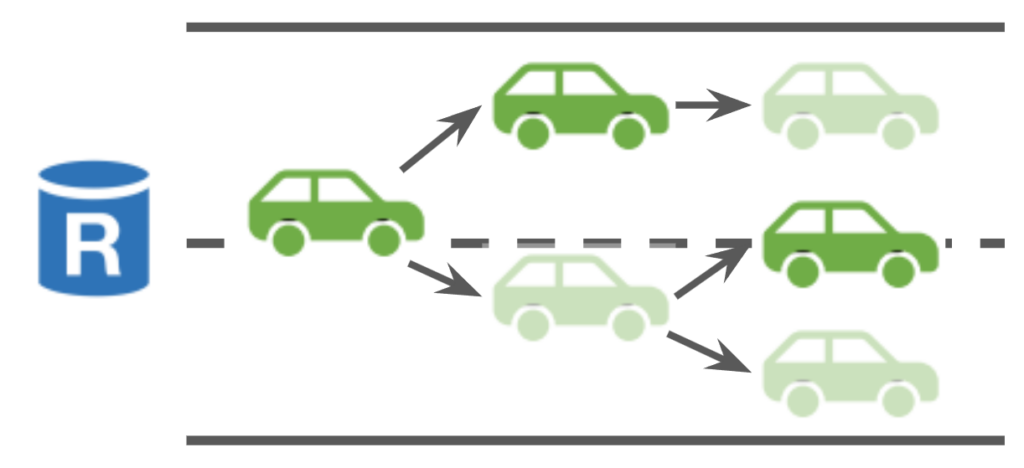
When this proposal is committed, the blocks in the proposed tip cut, along with all its parents up to the last tip cut (committed in the last consensus round), will be committed. This way, after recovering from a blip, a single round of consensus can commit all blocks disseminated during blips, and new requests will not observe any hangovers from here.
A minor problem with this design is that leaders across different views may choose tips from conflicting branches of a lane. In this case, instead of committing all ancestor blocks of the blocks in the current tip cut, Autobahn will only commit up to the block whose parent block is at the same height of the block in the previous tip cut. This means that not all committed blocks are on the same branch of the lane, but ideally this should only happen for Byzantine validators.
Committed blocks (in dark green) may be on different branches
The paper uses a linear PBFT-style protocol for consensus, where a round of consensus can be made in 1.5 round trips on the fast path and 2.5 round trips on the slow path. This latency can be reduced by using classic PBFT with all-to-all communication.
This article tries to summarize Autobahn, a new BFT protocol published in SOSP 24. The original paper can be found here: https://arxiv.org/abs/2401.10369
Background & Problem Statement
We first define a few terms to state the goal of this paper
Blip: periods during which protocol stops making progress. This includes network asynchrony and other events like when a Byzantine replica is selected as a leader.
Hangover: any performance degradation caused by a blip that persists beyond the return of a good interval. For example, after a blip, it takes time to process the client requests accumulated during blip, so new requests experience longer-than-usual delay. Some hangovers are unavoidable. E.g., even after network restoration, any protocol needs to wait until messages are delivered before making progress. Other hangovers are introduced by protocol logic and can be avoided with a better protocol design. These type of hangovers are refered to as protocol-induced.
Seamless: a partially synchronous system is seamless if (1) it experiences no protocol-induced hangovers and (2) does not introduce mechanisms (beyond timeouts necessary for liveness) that make the protocol susceptible to blips.
This paper tries to develop a low-latency seamless BFT protocol. Existing BFT protocols comes in 2 flavors:
Traditional BFT protocols (e.g., PBFT, HotStuff) assume a partially synchronous network where messages can be delayed up to some global stabilization time (GST). These protocols often involves a leader proposing a batch of requests (a block) and other replicas exchange vote messages to decide if the proposed block should be committed. This approach delivers low latency when network is stable by minimizing number of message exchanges between replicas. However, these protocols often suffer from hangovers due to queueing delay: when a blip ends, new transactions experience longer latency than usual as replicas try to clear up the requests accumulated during the blip. This hangover can be mitigated by proposing a huge batch of requests that includes all requests accumulated during blips and new requests, but sending such a huge batch is inherently slower than normal due to limited network bandwidth. If you always send such a huge batch then latency will increase as replicas need to wait for enough requests for a batch.
Direct Acyclic Graph (DAG) based BFT protocols (e.g., HoneyBadgerBFT, Tusk) assume asynchronous network. Each replica independently propose blocks through reliable broadcasts. Each block will point to some earlier blocks as its parents and thereby forming a DAG. To overcome FLP impossibility, these protocols use randomness when deciding if a block should be included in the final DAG. While they can immediately make progress when network restores, each reliable broadcast requires significant number of message exchanges, leading to high-latency. Furthermore, voting for a block often requires having all its ancestors. If a replica is missing some blocks, it may need to fetch them from others before they can vote for new blocks, leading to potential protocol-induced blips.
In summary, a seamless BFT protocol needs to:
Disseminate blocks asynchronously and independently from consensus ordering.
After a blip, either all blocks disseminated during blip can be committed immediately when they are delivered, or the replicas can start working on new requests as usual and the blocks disseminated during blip can be committed when the new requests are committed.
Replicas can vote even if it is missing some blocks.
Autobahn
Autobahn adopts the classic assumption of $n=3f+1$ where $n$ is the number of replicas and $f$ is the maximum number of faulty replicas it can tolerate. Autobahn is composed of a block dissemination layer and a consensus layer.
The block dissemination layer ensures that at least one correct replica stores the block so other replicas can always reliably fetch it as needed. In Autobahn, each replica independently batches the requests it receives into blocks and broadcast the block to other replicas in a propose message. Upon receiving a valid propose message from peers, the replica will respond with a vote message. When receiving $f+1$ votes for a proposal, replica can compose these $f+1$ votes into a proof of availability (PoA) indicating that this block is durably stored by at least 1 correct replica and everyone can reliably fetch the block whenever needed. The PoAs are sent to leader and passed to consensus layer. This process of proposing a block and composing the votes into its PoA is called Certification of Available Requests (CAR).
Certification of Available Requests (CARs)
CARs started by the same replica form the replica’s lane. Lastly, Autobahn adopts the chaining idea and each propose message includes the hash of its parent block (proposed by the same replica) and its PoA. When a replica receives a valid propose message, it will only respond with a vote if (1) it has voted for its parent block and (2) it has not yet voted for another block at the same height. However, since PoA only requires $f+1$ votes, there can still be multiple blocks, each with a PoA, at the same height, meaning that lanes can diverge. This is fine as the consensus layer will decide which branch of the lane will be committed.
Each replica has its lane and one CAR across each lane form a cut
Autobahn’s consensus layer follows a classic two-round linear PBFT-style agreement pattern. Instead of proposing blocks, the leader proposes one block with PoA from each lane, forming a lane cut. When a cut is committed, every block in the cut, along with its ancestors up to the previous cut, are committed. The ordering of these blocks are determined locally at each replica through some deterministic algorithm on the set of committed blocks. To achieve seamlessness, the proposed cut includes the PoA for the blocks to convince correct replicas that this cut is safe and they can fetch any missing blocks asynchronously after the blocks are committed. The consensus protocol proceed in (log) slots. For each slot, leader proposes a cut and wait for $2f+1$ votes from replicas indicating they locked in on this proposal (and they will not vote for another proposed cut for this slot) in the prepare phase. It then compose these votes into a quorum certificate (QC), send it to the replicas, and wait for their votes indicating that the decision is durably stored in the confirm phase. Finally, it composes votes from the confirm phase into another QC and send it to replicas for commit before moving to the next slot (5 message delays in total). As an optimization, if the leader receives all $n$ votes during the prepare phase, that means all $2f+1$ correct replicas have locked in for this proposal. When a view-change happens, the new leader will receive this proposal from at least $f+1$ correct replicas. This is sufficient to ensure that the proposed cut is durable and the confirm phase is not needed, enabling a 3-message-delay fast path.
Autobahn consensus
As with other BFT protocols with partial synchrony assumption, Autobahn relies on timeouts for liveness. If the leader does not propose for a while, replicas will send timeout message including the proposed cut in its last locked-in slot to the next leader. The consensus layer then proceeds as with the classic two-round linear PBFT. One important nuance is that, since lanes can diverge, the new leader may not agree with the old leader on the diverging blocks they have voted for during dissemination. As a result, the new leader may include a block in its proposed cut that does not extend from a block that has committed in the previous round by the old leader. In this case, replicas will only commit the ancestors of the new block whose heights are greater than the block in the last committed cut so that for each lane, only one block gets committed at each height, even if they do not necessarily extend from each other. Note that proposed cuts are monotonic since the latest cut replicas observe at the end of a slot instance is at least the proposed cut during the round.
Committed blocks in a lane. Dark green indicates that the block is committed.
Optimizations
Parallel Multi-Slot Agreement: In Autobahn, new slot instances can run in parallel with previous slots instead of having to wait for them to commit. Enabling such concurrent consensus requires a few modifications include: (1) when a proposed cut is committed at a slot, replicas need to wait for all the proposed cuts in the previous slots to execute before executing this one; (2) proposed cuts are no longer monolithic so replicas need to ignore out-dated blocks in the new cut; (3) leader do not need to wait for the previous cut to be committed before proposing a new cut, so timeout should start when the previous cut is proposed instead of when the previous cut is committed; (4) in case all parallel slot instances view-change through the same Byzantine leader, the leader election schedule for each instance is offset by $f$; (5) in case there are too many parallel instances during a blip, the number of parallel instances is restricted by some $k$, so slot instance $s$ cannot start until slot instance $s-k$ is committed. The paper points out that this approach is better than pipelining consensus phases (e.g., Chained HotStuff) as (i) this incurs lower latency since new proposals don’t need to wait for the previous phase to finish, (ii) this approach does not introduce new liveness concerns, and (iii) slot instances run independently and failing of one slot instance does not affect the progress of other slot instances.
Pipelining CARs: CAR for a new block can start without waiting for its parent block’s CAR to finish. Yet doing so means malicious validators can flood the network with blocks that will never commit.
Proposing Uncertified Cuts: Autobahn can further reduce latency by including blocks without PoA (uncertified blocks) in proposed cuts. One intuitive example is for leaders to include uncertified blocks in its own lane. Byzantine leaders may include unavailable blocks but correct replicas will simply realize that the block is unavailable when it tries to fetch the block and issue a view-change requests. A more aggressive approach allows the leader to optimistically include uncertified blocks from other validators. This approach hides two message delays (one for vote to the proposer and one for proposer sending the PoA back to leader) required for block dissemination from the critical path. However, this design sacrifices seamlessness as followers still needs to wait for PoA before voting. As a mitigation, during consensus, replicas can issue weak votes if it has not vote for another cut at the slot and strong votes if it additionally has the block data or PoA. This way, a quorum with $f+1$ strong votes can serve as its PoA.
Others: threshold signature to reduce size of quorum certificate; use all-to-all communication instead of linear to latency (each phase only incurs one message delay instead of two).
Strength
Autobahn achieves low latency. It only adds 3 message delays to the BFT protocol it uses for consensus. Client requests leader receives will experience 1 less message delay since it does not need to broadcast PoA. With the linear PBFT-style protocol it used in the paper, its latency is comparable with HotStuff.
Autobahn achieves high throughput. Its throughput is bounded by the block dissemination layer (no matter how fast block dissemination layer disseminates blocks, the consensus layer can always commit everything by voting on tip cut) and thereby achieve throughput comparable to DAG-based BFT protocols like Bullshark.
Autobahn is free from censorship: blocks proposed by any validator will eventually get included in some cut proposed by a correct leader. This design also provides basic chain quality as blocks by benign validators will be included on chain eventually.
Autobahn is resilient to blips: The only source of hangover left is that new requests may experience additional queueing delays if the receiving validator is waiting for its lane tip to get certified. However, to remove this hangover, the validators need to be able to start CARs unboundedly, and Byzantine validators may be able to flood the network with invalid blocks.
Weakness
Autobahn’s network complexity is higher than normal BFT protocols, as the message size of proposed cut has complexity of $O(n)$. This can limit its scalability. One may argue that Autobahn can commit much more than $n$ blocks in one consensus round (compared with HotStuff where each round trip only commits one block), and consequently validators actually exchange less bytes of messages to commit these blocks. However, this is only true if the leader has waited for long enough so that sufficiently many blocks have been disseminated between two rounds of consensus. Yet waiting for too long will lead to long latency. Care needs to be taken when pacing the consensus layer.
Profiling systems typically fall into one of the two categories. The first group uses binary modification, compiler support, or direct simulation of programs to gather measurements. They introduce significant overhead and usually require significant user intervention, so they are not deployed on production systems. The other group uses statistical sampling to collect fine-grained information on program or system behavior. They incur much smaller overhead but relies on existing source of interrupts (e.g. timer interrupts) to generated samples. This prevents them from sampling within those interrupt routines and can result in correlation between sampling and other system activity (bias).
The profiling system presented in this paper falls into the second category. It consists of two parts: a data collection subsystem that runs during program execution, and a suite of analysis tools that analyzes the collected data.
The data collection subsystem consists of 3 interacting components: a kernel device driver that services performance counter interrupts; a user-mode daemon process that extracts samples from the driver; and a modified system loader and other mechanisms for identifying executable images and where they are loaded by each running process.
First, each processor generates a high-priority interrupt after a specified number of events have occurred. The kernel device driver handles this interrupt by recording the PID of the running process, the program counter (PC), and the event type causing the interrupt. Since interrupts are frequently issued, the kernel device driver needs to handle them quickly. The driver keeps a per-process hash table to keep track of the number of times each (PID, PC, EVENT) tuple has occurred. This data structure avoids copying the recorded data to userspace on every timer interrupt. The hash table is implemented as an array of fixed size buckets. Whenever a new (PID, PC, EVENT) tuple is to be added to a full bucket, an old tuple in that bucket is evicted and copied to the user-mode daemon through a pair of overflow buffers. This basic design is efficient since it is cache friendly and synchronization is only needed when copying data into buffers. This paper handles this synchronization through inter-process interrupts. The user-mode daemon will map the events to the corresponding location in the executable image (through PID and PC) and store the records to disk.
After the samples are collected through the data collection subsystem, the analysis tool can be used offline to analyze the profiling results. It will identify for each instruction a frequency (number of times it is executed for a fixed time period), a cpi (average number of cycles spent in one execution), and a set of culprits (possible explanations for any wasted issue slots).
Estimating frequency and cpi is tricky since the data collection subsystem only shows the amount of time spent in this instruction relative to overall execution time, indicated by the sample count. More specifically, for each instruction $i$, its frequency $F_i$, cpi $C_i$, and sample frequency $S_i$ should satisfy $F_i\cdot C_i=S_i$. $S_i$ can be calculated directly from the sampling result. The analysis tool estimates $F_i$ through the following: it first does a static analysis on the program to identify the instructions that are guaranteed to execute for the same amount of time (i.e. basic blocks). This splits the program into a control-flow graph of basic blocks. It then runs each basic block $I$ individually to obtain an approximate $\sum_{i\in I} C_i$. Then the estimated frequency is $F_j=\sum_{i\in I} S_i/\sum_{i\in I} C_i$ for any instruction $j\in I$. Then it can calculate each $C_j$ accordingly.
To find the list of all possible culprits, this paper separately discusses static and dynamic causes. For static causes, it schedules instructions in each basic block using an accurate model of the processor issue logic and assume no dynamic stalls. With detailed record-keeping and accurate model, it is able to identify the static causes. For dynamic causes, it uses different techniques for each cause to check if it is possible that the dynamic stall is caused by this.
Anderson, Jennifer M., et al. “Continuous profiling: Where have all the cycles gone?.” ACM Transactions on Computer Systems (TOCS) 15.4 (1997): 357-390.
This paper presents Highly Available Network File System (HA-NFS). It splits the availability problem in to 3 kinds of availability problems and uses different strategies to improve each kind: server availability, disk availability, and network availability. This paper has three main goals: 1. failure and recovery should be transparent to the clients; 2. failure-free performance is unaffected (small overhead); 3. backward compatible with NFS clients.
Server availability is enhanced through primary-backup pairs. In HA-NFS, NFS servers are arranged in pairs connected to the same set of dual-port disks. They each serve as independent NFS servers during normal execution and both act as the backup for the other. Each server has two network interfaces: a primary and a secondary interface. Client requests are sent to the primary interface. On normal operation, an NFS server persists the requests it receives to a designated log disk. It also exchanges heartbeat with its partner server to monitor its liveness. If the partner server has not sent any heartbeat for a timeout period, the server sends an ICMP echo packet to the partner server, and then send a request through the dual-port disk if it still does not respond to the ICMP echo packet. Notice that both ICMP packet and the dual-port message passing trigger a high-priority interrupt on the partner server. This checks if the partner server is actually dead or is just busy processing other requests.
If the server determines that its partner server has failed, it starts a take-over process. It runs the logs and restore the filesystem to a consistent state. Then it changes the IP address of its secondary interface to that of the primary interface on the failed server. This reroutes the requests to the failed server to the live server. When the failed server comes back up, it uses its secondary interface to send reintegration requests to the live server. The live server will first unmount the corresponding filesystem, switch its secondary interface back, and ack back to the reintegrating server. The reintegrating server will then reclaim the disk, run logs to reconstruct the state, and switch its primary interface on. This protocol ensures an important safety invariant: at any point there is only one server working with one disk, so that there is no race condition.
Fast recovery from disk failures are achieved by mirroring files on different disks (RAID 1). Notice that the duplicated disks are managed by the same server, so there is no need for network round trips to ensure consistency.
HA-NFS relies on replicating network components to tolerate network failures. Each server has its primary and secondary network interfaces attached to different networks, and the two servers in the same primary-backup pair have their primary interface attached to different networks for load balancing. However, to recover from network failures, the client needs to detect the network failures to reroute the requests. In this design, the servers will broadcast heartbeat messages through its primary interface and a daemon on every client will detect the heartbeats. Notice that this configuration can tolerate the combination of server and network failures: in that case the live server’s network interface attached to the working network will take all the requests for the live and failed server.
Strength
This design is able to provide high availability with minimal cost. Each server is only doing more work in sending heartbeats and replicating the files to the backup disk.
In this design, all nodes are fully utilized, unlike primary-backup where the backup nodes never handle any requests when the primary is live.
Weakness
This design only permits one failure for each pair of servers. This availability guarantee is rather weak compared with primary-backup.
Backup takeover takes about 30 seconds and reintegration takes 60 seconds, which is extremely slow considering that no client requests can be processed during takeover and reintegration.
Bhide, Anupam, Elmootazbellah N. Elnozahy, and Stephen P. Morgan. “A highly available network file server.” USENIX Winter. Vol. 91. 1991.
Existing DNN frameworks manages the DNN operators in a data flow graph. The library (e.g. PyTorch) schedules each operator individually and relies on the hardware scheduling (e.g. cuDNN) to exploit parallelism within operators. This two-layer scheduling scheme works well only when the kernel launching time is largely negligible compared to execution time and when there is sufficient intra-operator parallelism to saturate all processing units, but precludes opportunities to run multiple operators in parallel on the same GPU.
(a) shows the two-layer scheduling approach; (b) is a more efficient scheduling plan. Notice that this more aggressive plan requires that Operator 0 and 1 do not depend on each other.
Rammer is a deep learning compiler aimed to unify the inter- and intra-operator scheduling. It defines each DNN operator as rOperator and splits the rOperators into rTasks. A rTask is the smallest unit of scheduling and will run on a single processing unit (e.g., SM in GPU). We can think of rTasks as thread blocks. Rammer also introduces a special rTask, namely barrier rTask, that stalls execution until a set of rTasks has completed. Another abstraction that Rammer provides is rKernels, which corresponds to the actual implementation of rOperators (e.g., if the rOperator is convolution, then rKernel can be matrix multiplication, FFT, etc). Notice that different rKernels will split the rOperator into different rTasks.
Rammer abstracts the hardware as a virtualized parallel device (vDevice, corresponding to GPUs) composed of multiple virtualized execution units (vEU, corresponding to the SMs). This paper achieves single-layer scheduling by assigning rTasks to different vEUs at compile time, and then pin the compiled vEUs on the hardware processing units. From the DNN model, Rammer generates a static execution plan. This plan is broken into multiple parts called rProgram, which is represented as a 2D array of rTasks where the first index represents on which vEU this rTask is assigned to and the second index represents the order in which it will be run on that vEU. Each rProgram runs on a single rDevice. Rammer thereby achieves scheduling over multiple hardware devices (GPUs).
Rammer architecture. Accelerator refers to the hardware processing units.
The architecture of Rammer is shown in the figure above. After obtaining the DNN model, Rammer first transforms it to a DFG of rOperators. It does some compile-time profiling to figure out which rKernel is the most efficient through profiling and heuristics. Then the rOperator can be split into rTasks. Rammer uses a Wavefront Scheduling Policy, which is essentially a BFS on the DFG of rOperators. Here wavefront refers to the rTasks that do not depend on any other unscheduled rTasks. The policy iterates through the rTasks in the wavefront and assigns the current rTask to the vEU that becomes available first (based on profiling results). However, if the profiling result shows that assigning the current rTask to the current rProgram does not save execution time, it will put the rTask to a new rProgram that will be run on a different vDevice instead.
Strength
Rammer exploits the inter- and intra-operator parallelism holistically. It can provide higher GPU utilization compared with traditional two-level scheduling
The scheduling plan is statically generated, so it does not impose any runtime overhead.
Weakness
Rammer is only beneficial when there is not sufficient intra-operator parallelism (e.g. in inference workloads) or when the kernel launching overhead is largely negligible. Yet often times neither is true in typical training workloads.
Rammer can only parallelize two operators if they are independent. With linear models (e.g, ResNet) there is not much Rammer can do.
Rammer generates scheduling plan statically. If the underlying hardware changes dynamically (e.g., shared between multiple models in data centers), it cannot adapt to the changes.
Ma, Lingxiao, et al. “Rammer: Enabling Holistic Deep Learning Compiler Optimizations with {rTasks}.” 14th USENIX Symposium on Operating Systems Design and Implementation (OSDI 20). 2020.
For distributed systems it is useful the know the global state at some point of time for various tasks like deadlock detection. However, in absence of synchronized clocks, it is hard to obtain a snapshot of the current state of the distributed system without stopping it since they might all take a snapshot at a slightly different time, leading to inconsistency. In this paper, snapshot contains the local state of each node and the messages sent between nodes. So a simple inconsistency can be that the sender records the state before a message is sent but the receiver records the state after the message is received, leading to duplicated message passing.
To begin, this paper makes the following assumptions:
Messages are never dropped or reordered.
The network delay is finite.
Then the snapshot algorithm runs as follows: first, processes periodically decide to initiate a snapshot. After it is done sending messages to other processes, it records its local state and sends a marker along the channels to indicate that the messages are sent before the snapshot. The receiver, upon receiving the marker, will record its local state if it has not yet done so, and record the messages in channel where the marker comes from since the state has been recorded. It will also broadcast the marker if it has not yet done so. The algorithm will terminate once all processes has recorded its local state and each channel has transmitted one marker.
An important property of this algorithm is that the recorded state may have never actually occurred during the execution: it simply records a state consistent with the partial order of events. This is because we can get a consistent snapshot regardless of in which order the concurrent events occur.
M. Chandy and L. Lamport. Distributed Snapshots: Determining Global States of Distributed SystemsLinks to an external site.. ACM Trans. Comput. Syst., 3(1):63-75, 1985.
In a distributed system, the notion of physical time is weak since each node has its own clock. Hence we need a different way to obtain an ordering of events and a clock that all nodes agree upon independent of each node’s internal clock. In this paper, we assume that sending a message and receiving a message are two events. This allows us to obtain a partial order independent of the physical clock. In particular, $\rightarrow$ is defined s.t., for any two events $a$ and $b$, $a\rightarrow b$ if and only if:
$a$ and $b$ happens within the same process and $a$ happens before $b$
$a$ is sending a message and $b$ is receiving the same message
There is another event $c$ s.t. $a\rightarrow c$ and $c\rightarrow b$
Notice that this ordering definition is only a partial ordering. If for two events $a$ and $b$ s.t. neither $a\rightarrow b$ nor $b\rightarrow a$, then we say they are concurrent.
Using this ordering definition, we can define logical clocks. Let $C_i(a)$ be the clock time on process $i$ that event $a$ happens and let $C(a)$ be the clock time of the entire system that event $a$ happens (if $a$ happens on process $i$, then $C(a)=C_i(a)$). In order for the clock to realistically reflect the ordering of events, it needs to follow the clock condition: for any events $a$, $b$, if $a\rightarrow b$ then $C(a)<C(b)$. Notice that the converse is not true since the two events may be concurrent. To satisfies the clock condition, it is sufficient if the logical clock satisfies that
If $a$ and $b$ happens on the same process $i$ and $a$ comes before $b$, then $C_i(a)<C_i(b)$
If $a$ is the sending of a message from process $i$ and $b$ is the receiving of the same message from process $j$, then $C_i(a)<C_j(b)$.
The algorithm hence does the following:
Each process increments its local clock for each event it encounters.
Each message are tagged with a timestamp of the sender. When a process receives a message from another process, it sets its local clock to be greater than the attached timestamp from the sender and greater than or equal to its current local timestamp.
With such a logical clock, we can construct a total ordering ($\Rightarrow$) of all events. Let $<$ be an arbitrary order on the processes, then for any two events $a$, $b$, $a\Rightarrow b$ if and only if $C_i(a)<C_j(b)$ or $C_i(a)==C_j(b)$ and $P_i<P_j$. Notice that all processes will reach the same ordering of all events, so synchronization is achieved.
One problem remaining is that, with a logical clock, the distributed system is not aware of the time of external events. For example, if client $A$ sends a request before client $B$ but $B$’s request arrives at the distributed system before $A$’s, then the distributed system will order $B$’s request before $A$’s. To avoid this, physical clocks are needed. In order to build a physical clock, it is necessary that each node’s internal clock must be running at approximately the correct rate, and that all nodes are at an approximately same time at any moment. Formally, the physical clock $C_i(t)$ ($t$ is the actual time) at any node $i$ must satisfy that
There exists a constant $\kappa \ll 1$ s.t. $|\frac{dC_i(t)}{dt}|<\kappa$.
There exists a small constant $\epsilon>0$ s.t. $|C_i(t)-C_j(t)|<\epsilon$.
The first condition is achieved through hardware: for typical crystal controlled clocks, $\kappa\le 10^{-6}$. To achieve the second condition, each process $i$ includes in each message $m$ it sends with the current timestamp $T_m=C_i(t)$. Upon receiving a message at time $t’$, the receiver process $j$ will update its clock to $max\{C_j(t’), T_m+\mu_m\}$ where $\mu_m\ge0$ is the minimum network delay (i.e. $t’-t\le\mu_m$).
Vector Clocks
There are, however, some disadvantages in the logical clock defined in this paper. Recall that when $C(a)<C(b)$, we cannot determine that $a\rightarrow b$ since they might be concurrent. But such information is lost in the logical clock, and many concurrent events now look like $a\rightarrow b$. This leads to more conflicts, making it harder to track events with actual dependency. To resolve this, a commonly used clock in distributed systems nowaday is the vector clock. Here, each process $i$ locally keeps a list of clocks $C_i = \langle c_1, c_2, …, c_n\rangle$, one for each process in the distributed system with $n$ processes. This clock is updated as follows:
For local operations, the process $i$ simply increments its own counter $C_i[i]++$.
When sending a message, in addition to incrementing its own counter $C_i[i]++$, it will also send the updated $C_i$ (all $n$ clocks) along with the message.
Upon receiving the message, the receiver $j$ will first update its own counter $C_j[j]++$. Then, for $k=1,…,n$, it updates the local clock by $C_j[k] = max\{C_j[k], C_i[k]\}$.
Then for any two events $a$ and $b$, the ordering is defined as
$C(a)\le C(b)$ if $C(a)[i]\le C(b)[i]$ for all $i$
$C(a)<C(b)$ if $C(a)\le C(b)$ and that $C(a)[i]<C(b)[i]$ for some $i$.
A noticeable drawback of vector clocks is that each process is locally keeping a clock for all other processes, leading to higher space overhead. Additionally, it also makes it harder for nodes to enter and exit the distributed system since that means we need to dynamically allocate space for more clocks on each node.
L. Lamport. Time, Clocks, and the Ordering of Events in a Distributed SystemLinks to an external site.. Communications of the ACM, July 1978, pages 558-564.
Low-Bandwidth Filesystem (LBFS) is a network file system designed to run in presence of network with low bandwidth, which is common when the client and server are remotely located. LBFS is based on NFS v3. A key observation is that, in most cases, a file is only modified slightly, while existing network filesystems retransmit the entire file every time. To reduce the amount of data sent over the low-bandwidth network, LBFS only sends data if it is not present on the other side of connection.
In LBFS, each file is divided into chunks using a sliding window of 48B. Whenever (the lower 13 bits of) the fingerprint of contents in the 48B window matches a certain value, it becomes a breakpoint that separates two chunks. This has two important benefits: 1. it is resistant to insertions; 2. chunks with the same data will have the same breakpoints, so chunks divided in this way are more likely to contain the exact same data. To prevent some pathological cases, LBFS breaks a chunk if it is too large (64K) and prevents breaking if a chunk is too small (2K). LBFS uses SHA-1 hash and a local database to detect duplicate data chunks. LBFS stores in the database the location of each chunk indexed by its SHA-1 hash value (SHA-1 is collision resistant). To reduce the overhead of maintaining the database, it is not updated synchronously during writes. Although this can lead to inconsistency, LBFS does not rely critically on the correctness of the database and will check if the data actually matches the hash on each access.
The LBFS protocol is based on NFS v3 adding lease support. It performs whole-file cache. When a client makes any RPC on a file, it is granted a read lease. If an update occurs during the lease period, server will notify the client about it. After the lease expires, the client needs to check with servers for the attributes of the file for consistency, which implicitly grants the client a read lease. LBFS thereby provides a close-to-open consistency. Similar to AFS, however, LBFS caches all updates locally until the file is closed, during which all updates are atomically written back in the server. Hence, in presence of concurrent writers, the last one to close a file will overwrite the modification made by others.
LBFS avoids transmitting data that are already present on the other side. During a read or write, the sender will first break the file into chunks, find the SHA-1 hash of each chunk, and check with the receiver if the same chunks are present on its side. The sender will only send the chunks missing from the receiver side. Below are the routines for reading and writing a file in LBFS. One may notice that during write, the new file is written to a temperate file that will replace the original file atomically when the write completes.
Reading a file in LBFSWriting a file in LBFS
Strength
The use of fingerprint to identify chunks with similarities and use SHA-1 to find duplicate is simple and neat in reducing the data transmitted through the network.
From evaluation LBFS is able to identify 38% overlapping data within some object files containing metadata, and 90% overlapping data for human readable documentations in normal workloads, significantly reducing the amount of data getting transmitted.
Weakness
LBFS relies critically on that SHA-1 is collision resistant. If two chunks happen to have the same hash value, only one will be kept on the server. This means a malicious user can do the following:
Uploading chunks with various hash value to infer if a certain chunk of data is present on the server
Uploading a huge amount of chunks with various hash value so that future files uploaded by other users containing a chunk with the same hash value will be polluted.
Muthitacharoen, Athicha, Benjie Chen, and David Mazieres. “A low-bandwidth network file system.” Proceedings of the eighteenth ACM symposium on Operating systems principles. 2001.
Coda builds on AFS to improve availability by leveraging file caches on clients. It behaves like AFS when client is connected to the server to retain the high scalability of AFS.
Coda introduces some new concepts: disconnected operations, which are the operations performed when client is disconnected from the server. When a client is disconnected from the server, disconnected operations on the local cache can still be performed. The operations are logged locally and are sent to the server when the connection is restored. Coda thereby achieves high availability. Coda also introduces volume storage group (VSG), or the set of replication sites of a volume (i.e. the servers with a copy of the volume).
One major difference of Coda from AFS is that, instead of assigning each file a server responsible for all updates to that file, Coda allows updates to be made on more than one server with a replicated file, which will propagate the changes to other replications. During a disconnection, a client may have access to only a subset of a VSG, which we term accessible VSG (AVSG). In Coda, modifications are first sent to AVSG from the client, and eventually propagated to the missing VSG sites. This paper did not mention what happens in presence of concurrent updates to different servers.
When disconnected from the servers, Coda relies on the locally cached copy of files for update. At any moment a Coda client must be in one of the three states: hoarding state, where the client is still connected to the server and performs like AFS; emulation state, where the client is disconnected from the server; reintegraton state, where the connection is restored and client needs to resynchronize with the server (in AVSG).
During the hoarding state, Coda behaves normally as AFS in that it performs all updates on local cache and send the update to the server on close. However, since disconnection can happen anytime, we want to make sure that the files that are most likely be used during a sudden disconnection are cached locally. Coda hence manages the cache using a prioritized algorithm. The key idea is that the users can assign each file different hoard priorities and the prioritized algorithm will evaluate the current priority of a cached object based on its hoard priority and recent usage. Notice that since a file’s current priority changes over time (since it relies on recent usages), it is possible that a file cached locally has lower priority than a file not cached (e.g. File A has a hoard priority of 5 and is not used while File B has a hoard priority of 0 but is used recently: File B will have a higher priority after use but gradually File A will have a higher priority). To compensate this, the client does a hoard walking that reevaluates the priority of each file and replace the caches. Finally, to open a cached file, the client will still have to perform a path resolution, so the parent directories of a cached file cannot be evicted before the cached file gets evicted.
When the client is disconnected, it enters the emulation state, during which it will perform actions normally handled by the servers. This include creating a new file, during which it will generate dummy file identifiers (fids). During the emulation state, all requests are performed against the cached local copy instead of going to the Coda server, so requests on a file not cached locally will fail. The Coda client keeps a replay log locally that contains enough information to replay the updates on the server. Lastly, since we no longer have the remote copy, all modified files are kept in cache with highest priority and are flushed more frequently.
When the connection is restored, the client enters a reintegrations state. The client will first request fids for newly created files from the Coda server, then send the replay log to each server in AVSG in parallel. The Coda server, upon receiving the replay log, will perform the replay algorithm one volume at a time. For each volume, it will first parse the replay log, lock all objects referenced, and validate and execute all operations in the log. Then the actual data are transferred from client to server (a.k.a back-fetching). Finally it will commit the updates in one transaction (per volume) and release all locks. However, replay may fail because another update to the same file occurred during disconnection. Coda asks the client to locally resolve any conflicts in updates.
Strength
Coda makes the file available during disconnection at a low cost.
Similar to AFS, Coda is scalable since most operations on the critical path are performed locally.
Weakness
Similar to AFS, Coda is not good at sharing.
Coda caches objects at the granularity of a whole file. This is not friendly for huge files or if the client only need a small portion of a file.
Coda is not very graceful during emulation state if the disk resource at client is exhausted.
Satyanarayanan, Mahadev, et al. “Coda: A highly available file system for a distributed workstation environment.” IEEE Transactions on computers 39.4 (1990): 447-459.
Andrew File System (AFS) is a distributed filesystem designed and implemented in 1980s after NFS v2. It focuses on improving the scalability by resolving 3 problems: 1. reduce the amount of requests sent to the server; 2. reduce the amount of computation (e.g., pathname resolution, context switch, etc) on the server; 3. load balancing between multiple AFS servers.
AFS servers are leader based: each file stored in AFS is replicated over multiple nodes with one dedicated leader. All update requests to the file are directed to the leader node that will propagate the update to all other read-only replicas. When the client accesses a file, it fetches it from the server and keeps a local cache. When it tries to access the same file again, it will check with the server responsible for that file if the file has recently been modified. If not, it will use the local cache instead of fetching the file from the server again. This provides a simple close-to-open consistency guarantee.
An important feature of AFS is that for a typical read-modify-write operation on a file, an AFS client simply requests the entire file from the server on opening, apply all updates to its local cache, and commit the changes to the server on closing. This significantly reduces the number of requests sent to the server from a client: regardless of the number of operations between open and close, only two requests are communicated to the server. However, this also means that updates are only visible to other clients on close, so if there are multiple clients concurrently updating the same file, the last one that commits will overwrite all updates from other clients. AFS assumes that concurrent access is rare and requires application level concurrency control for sharing.
AFS improves performance through caching: if a file is already present in cache, it does not have to request it again from the server. Yet, instead of periodically checking with the server for validity, AFS uses callbacks: when the client requests a file, the server attaches a callback to that request. When a client commits some updates to a file, the server breaks the callbacks to notify all other clients that their caches are no longer up-to-date. Hence if a cache has a callback, the client can assume that this file has not been modified and use it directly.
AFS servers manage files using key-value stores. Each file on AFS is associated with a unique fixed-length Fid and directories map pathnames to the corresponding Fids. The clients will locally resolve for the Fid corresponding to the desired pathname with its local directory cache and present the Fid to the server. The server manages files in volumes: Fid contains information about which volume the file belongs to, its offset within the volume, and a uniquifier that indicates if the file corresponding to that Fid is still the original file, not a different file placed in the same position in the same volume after the original file was removed. AFS achieves load balancing by moving volumes among the servers. A distributed database keeps track of on which server each volume is located.
Strength
The design of AFS delivers high scalability: the client only communicates with the server for open, close, and other operations off the critical path, significantly reducing the server load when compared with NFS.
Changes to a file are materialized atomically on close, making it easy for failure handling: only server or client failure during close may lead to crash consistency issues. The server contains a consistent copy at any other time.
The abstraction of volume makes data migration (and hence load balancing) simple, and files are still accessible during volume migration.
Weakness
This design makes sharing complicated. Modifications on one client is not visible on other clients until it closes the file, and AFS relies on application-level concurrency control permit sharing.
AFS clients always cache the entire file. If the client only needs to access a small portion of a large file, this can incur huge network traffic and exhaust client storage resources.
John H Howard, Michael L Kazar, Sherri G Menees, David A Nichols, MahadevSatyanarayanan, Robert N Sidebotham, and Michael J West. 1988. Scale andperformance in a distributed file system.ACM Transactions on Computer Systems(TOCS)6, 1 (1988), 51–81.